Geospatial Concepts & Glossary
Introduction
This page provides foundational knowledge for working with geospatial marine data. If you’re new to spatial analysis or need a refresher, start here before diving into the tutorials.
Spatial Data Types
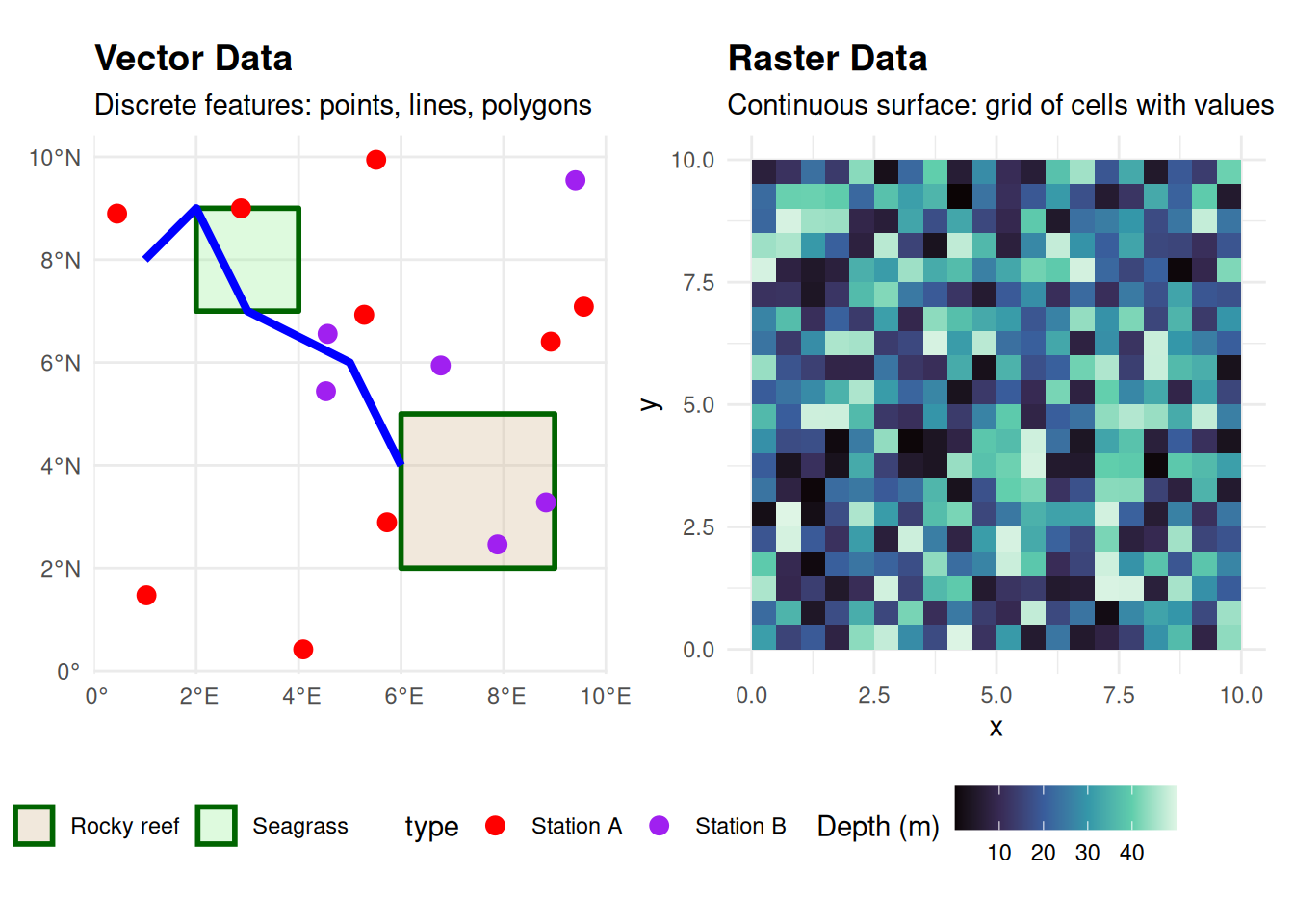
Geospatial data comes in two fundamental forms: vector and raster (Figure 1). Understanding the difference is crucial for choosing the right analysis methods.
Vector Data
Vector data represents discrete geographic features as points, lines, or polygons. Each feature has a precise location and can carry associated attributes (metadata).
Common vector data types:
- Points - Specific locations (e.g., species observation sites, sampling stations, platform locations)
- Lines - Linear features (e.g., ship tracks, transects, pipelines)
- Polygons - Enclosed areas (e.g., marine protected areas, habitat boundaries, survey regions)
Examples in EMODnet:
- Marine protected area boundaries
- Species occurrence records
- Subsea infrastructure (pipelines, cables)
- Habitat classification polygons
- Survey locations
Vector data is ideal when you need exact boundaries, discrete locations, or want to perform operations like counting features or measuring precise distances.
Raster Data
Raster data represents continuous spatial phenomena as a grid of cells (pixels), where each cell contains a value representing a measurement or category.
Common raster characteristics:
- Organized as rows and columns of cells
- Each cell has a specific resolution (size)
- Values can be continuous (e.g., depth, temperature) or categorical (e.g., habitat types)
- Often used for environmental variables
Examples in EMODnet:
- Bathymetric depth models
- Species abundance grids
- Habitat suitability indices
- Environmental variables (temperature, salinity)
- Derived biodiversity metrics
Raster data excels at representing continuous surfaces, enabling analyses like extracting values at points, calculating zonal statistics, or modeling spatial patterns.
Web Services for Spatial Data
What is a Web Service?
A web service is a standardized protocol that allows software applications to communicate with databases over the internet. In the context of spatial data, web services provide programmatic access to spatial databases - you send a request (e.g., “give me species observations in this bounding box”) and the service queries its database and returns the data.
Essentially, web services are spatial databases + standardized communication protocols that let you query and retrieve data through HTTP requests instead of needing direct database access.
Key benefits:
- Programmatic access - Query data directly from R without manual downloads
- Selective retrieval - Request only specific regions, time periods, or attributes
- Always current - Access the latest data without managing file versions
- Reproducible - Your code documents exactly what data was retrieved
- Efficient - Download only what you need, reducing bandwidth and storage
How Web Services Work
Figure 2 illustrates the typical workflow when accessing EMODnet data through web services.
flowchart LR
    A[Your R Script] -->|HTTP Request<br/>bbox, layer, filters| B[EMODnet WFS/WCS Server]
    B -->|Query| C[(Spatial Database)]
    C -->|Matching Data| B
    B -->|Response<br/>GeoJSON/GeoTIFF| A
    A -->|Load into| D[R Object<br/>sf or terra]

    style A fill:#e1f5ff
    style B fill:#fff4e1
    style C fill:#f0f0f0
    style D fill:#e1f5ff
OGC Standards and Spatial Data Types
The Open Geospatial Consortium (OGC) has developed different standard protocols optimized for different types of spatial data. The protocols, underlying database technologies, and data formats all differ based on whether you’re working with vector or raster data.
EMODnet provides two primary types of OGC-compliant geospatial web services, each designed for a specific spatial data type:
WFS (Web Feature Service)
WFS delivers vector data: discrete geographic features with attributes.
Key characteristics:
- Returns features in formats like GeoJSON or GML
- Supports spatial and attribute filtering
- Allows querying specific areas or feature properties
- Ideal for points, lines, and polygons
In R: Use the emodnet.wfs package to access WFS services. The package simplifies discovering available layers, filtering by extent or attributes, and retrieving data as sf objects.
What information can you access?
Before downloading data, WFS services let you discover which feature types (layers) exist and what attributes each layer contains. Once you retrieve data, you receive discrete geographic features (points, lines, polygons) with associated attributes describing those features (e.g., species observations with taxonomic details, protected area boundaries with designation information, infrastructure with operational attributes).
Example WFS data from EMODnet:
- Species occurrences and distributions
- Marine protected area boundaries
- Infrastructure features (platforms, pipelines, cables)
- Habitat polygons
WCS (Web Coverage Service)
WCS delivers raster data: gridded coverage representing continuous variables.
Key characteristics:
- Returns coverage in formats like GeoTIFF
- Supports spatial and temporal subsetting
- Can extract specific bands from multi-band datasets
- Ideal for environmental layers and modeled surfaces
In R: Use the emodnet.wcs package to access WCS services. The package handles coverage discovery, spatial/temporal subsetting, and returns data as terra raster objects.
What information can you access?
Before downloading data, WCS services provide metadata about available coverages: which datasets exist, their spatial and temporal extent, resolution, coordinate reference systems, and what bands/variables each coverage contains. When you retrieve data, you receive gridded rasters where each cell contains measurements or modeled values for continuous variables (e.g., bathymetric depth, species abundance predictions, habitat suitability indices, environmental measurements).
Example WCS data from EMODnet:
- Bathymetric depth models
- Species abundance and diversity grids
- Habitat suitability models
- Gridded biodiversity metrics
Advantages of Web Services
Compared to direct file downloads, web services offer:
- On-demand access - Get only the data you need, when you need it
- Spatial filtering - Request data for specific regions using bounding boxes
- Temporal subsetting - Extract data for particular time periods
- Always current - Access the latest data without managing downloads
- Reproducibility - Script your data access for transparent, repeatable workflows
Coordinate Reference Systems (CRS)
A Coordinate Reference System defines how coordinates relate to locations on Earth’s surface. Understanding CRS is essential for accurate spatial analysis.
The Challenge: From 3D Earth to 2D Maps
Earth is a three-dimensional sphere, but maps and computer screens are two-dimensional. Think of trying to peel an orange and flatten the peel completely - you can’t do it without distorting, stretching, tearing, or overlapping parts of it. This is the fundamental challenge of cartography.
Projections are different methods of “peeling and flattening” Earth’s surface. Just as there are many ways you could cut and flatten an orange peel (peel it in strips, cut it into wedges, try to keep it in one piece), there are many different projection methods, each making different choices about:
- Where to cut (what regions to split)
- What to stretch (which areas get distorted)
- What to preserve (angles, areas, distances, or shapes)
There is no perfect solution - every projection sacrifices something. This is why dozens of projections exist: each is optimized for different purposes and geographic regions.
NoteSpecifying CRS: EPSG Codes and WKT
Throughout this page, you’ll see CRS referenced by EPSG codes (e.g., EPSG:4326, EPSG:3857). EPSG stands for the European Petroleum Survey Group (now maintained by the International Association of Oil & Gas Producers), which created a standardized registry assigning unique numeric codes to coordinate reference systems. These codes provide a concise, unambiguous way to specify which CRS you’re using.
Under the hood, CRS definitions are stored as WKT (Well-Known Text) strings - a verbose text format that fully describes the coordinate system, datum, units, and other parameters. You’ll occasionally encounter WKT when inspecting spatial objects, but in practice you’ll usually work with EPSG codes which are simpler and map to the full WKT definitions.
Geographic vs Projected CRS
Geographic Coordinate Systems (Unprojected)
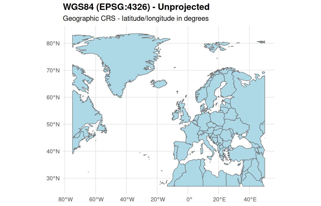
Geographic CRS don’t actually “flatten” Earth - they describe locations on the 3D spheroid surface using angles (latitude and longitude in degrees). Think of this as leaving the orange intact and describing locations by their angular position from the center.
- Example: WGS84 (EPSG:4326) (Figure 3 (a)) - Most common for global marine data and default for EMODnet services
- Units in degrees, not meters
- Good for storing and sharing data globally
- Not suitable for measurements - a degree of longitude represents different distances at different latitudes (degrees get closer together near the poles)
Projected Coordinate Systems
Projected CRS actually perform the “flattening” using mathematical transformations. Each projection is a different flattening method with different trade-offs:
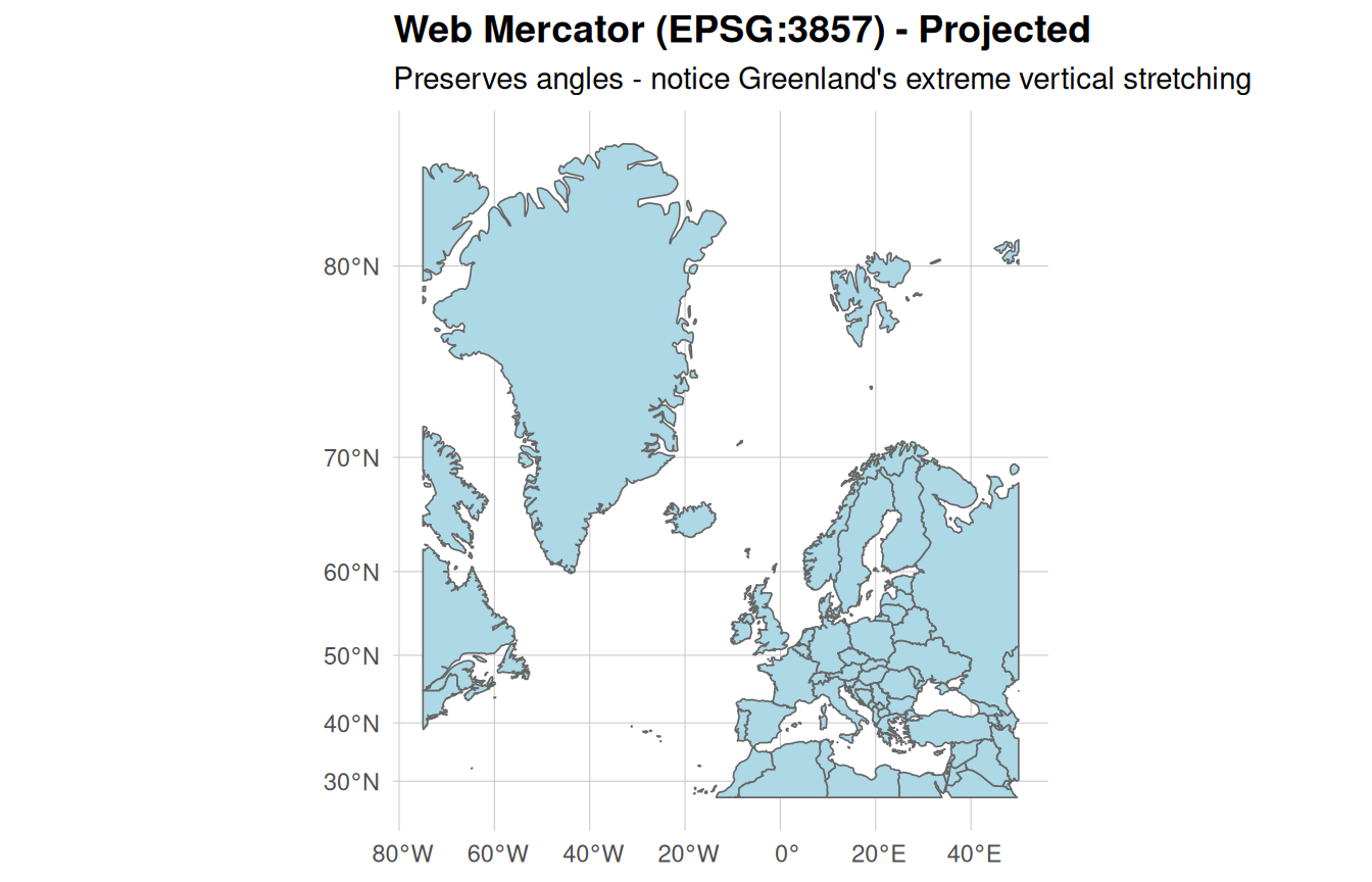
Web Mercator (EPSG:3857) (Figure 3 (b)) - “Peels the orange” by stretching areas increasingly toward the poles. Preserves angles (conformal projection), which historically made it invaluable for maritime navigation - sailors could plot a straight line between two points and maintain a constant compass bearing throughout their journey. However, this comes at the cost of severely distorting areas at high latitudes. Used by most web maps because it makes the whole world fit in a square.
UTM zones (e.g., EPSG:32631 for UTM 31N) - “Cuts the orange” into 60 vertical strips (zones), each 6° of longitude wide. Each strip is flattened with minimal distortion within that zone. Excellent for regional analysis.
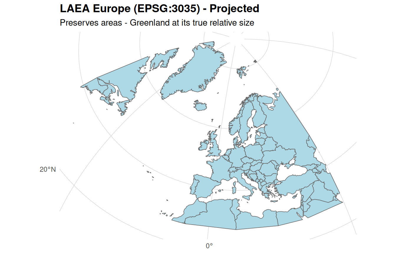
Lambert Azimuthal Equal Area (EPSG:3035) (Figure 3 (c)) - “Flattens the orange” while preserving area relationships. A 100 km² habitat appears as 100 km² on the map, regardless of location. Essential for statistical analyses involving area.
Local projections - Optimized flattening methods for specific countries or regions, minimizing distortion in areas of interest.
Figure 3 compares these three coordinate reference systems using Europe and Greenland to illustrate the dramatic differences in how projections distort geographic features.
Why This Matters for Marine Spatial Analysis
Measurements require projected CRS - You can’t accurately calculate distances or areas in degrees (geographic CRS). You need a projection that converts to meters.
Choose projections for your region - A projection optimized for Europe will distort tropical regions. Use UTM zones for your study area or regional equal-area projections.
Match your analysis goal - Use equal-area projections for habitat area calculations, equidistant projections for dispersal distance analyses, or conformal projections for angular relationships.
Alignment is critical - All datasets in an analysis must use the same CRS, or features won’t align correctly.
Working with CRS in R
Both major R spatial packages provide CRS transformation functions:
-
Vector data (sf) - Use
st_transform()to convert between coordinate systems -
Raster data (terra) - Use
project()to reproject raster layers
The tutorials demonstrate when and how to transform between CRS for different types of spatial analyses.
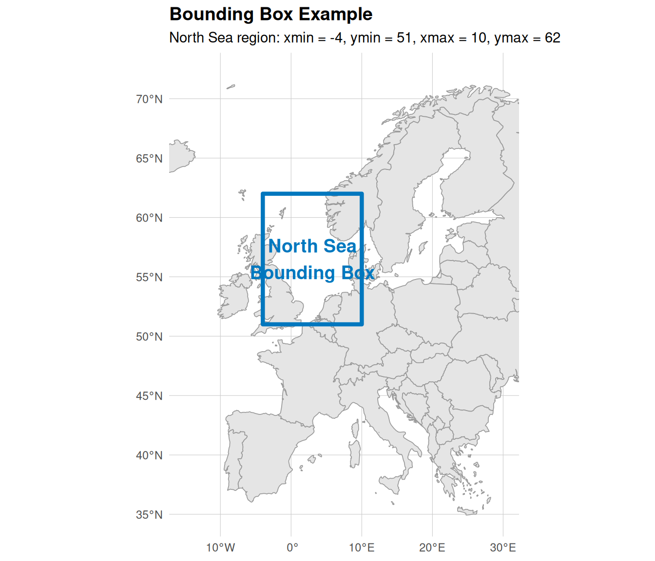
Bounding Boxes and Spatial Queries
A bounding box defines a rectangular area of interest using minimum and maximum coordinates (xmin, ymin, xmax, ymax). Bounding boxes are fundamental to spatial queries, allowing you to request only the data you need from web services rather than downloading entire datasets. Figure 4 shows a bounding box for the North Sea region.
Why Use Bounding Boxes?
Bounding boxes enable efficient spatial data retrieval by:
- Reducing data transfer: Download only features or coverage within your study area
- Improving performance: Smaller data volumes mean faster processing and lower memory requirements
- Focusing analyses: Limit results to relevant geographic regions from the start
- Reproducible workflows: Explicit spatial extent definitions make analyses transparent and repeatable
Bounding Boxes in EMODnet Services
Both WFS (vector) and WCS (raster) services accept bounding box parameters to spatially filter results. When querying EMODnet data through the emodnet.wfs and emodnet.wcs packages, you specify bounding boxes as numeric vectors with minimum and maximum coordinates. The coordinate reference system for bounding boxes should match the CRS of the data you’re requesting, which varies by layer.
The tutorials demonstrate practical bounding box usage for retrieving EMODnet data in specific regions, from local study sites to broader management areas.
The Geospatial Software Stack
Before diving into R packages, it helps to understand the foundational libraries that power geospatial computing. These open-source C/C++ libraries do the heavy lifting. R packages like sf and terra are interfaces that make them accessible from R.
Core Libraries
GDAL (Geospatial Data Abstraction Library)
GDAL handles reading and writing spatial data formats. When you load a GeoTIFF, GeoJSON, or Shapefile in R, GDAL is doing the work behind the scenes. It supports over 200 raster and vector formats, making it the universal translator for geospatial data.
- Website: gdal.org
PROJ
PROJ handles coordinate transformations and projections. When you convert data from WGS84 (latitude/longitude) to a projected coordinate system like UTM, PROJ performs the mathematical transformation. It maintains an extensive database of coordinate reference system definitions.
- Website: proj.org
GEOS (Geometry Engine - Open Source)
GEOS performs geometric operations on vector data: intersections, buffers, unions, validity checks, and more. It works with planar coordinates, treating geometries as flat 2D shapes and using Euclidean geometry. This is fast and works well with projected coordinate systems.
- Website: libgeos.org
s2 (S2 Geometry Library)
s2 is Google’s library for spherical geometry. Unlike GEOS, it treats the Earth as a sphere and performs calculations on the curved surface. This is appropriate for geographic CRS like WGS84 (EPSG:4326), where coordinates are in degrees. s2 is geometrically correct for unprojected data but slower than GEOS, stricter about geometry validity, and doesn’t support all operations (e.g., st_simplify() requires GEOS).
- Website: s2geometry.io
Why This Matters
Understanding this stack helps explain behaviours you’ll encounter:
GEOS vs s2: The
sfpackage uses s2 by default for geographic CRS and GEOS for projected CRS. Some operations only work with GEOS, which is why you sometimes seesf_use_s2(FALSE)in code to temporarily switch engines.CRS transformations: When you call
st_transform(), PROJ does the coordinate conversion.Format support: If R can read a spatial format, it’s because GDAL supports it.
The Stack in Practice
When you run a typical spatial workflow in R:
- Loading data: GDAL reads the file format
- Reprojecting: PROJ transforms coordinates
- Spatial operations: GEOS or s2 performs intersections, buffers, etc.
- Saving results: GDAL writes the output format
The R packages coordinate these libraries and provide a consistent interface, but the underlying work happens in optimised C/C++ code.
Key R Packages
sf - Simple Features for R
The sf package is the modern standard for vector spatial data in R. It provides an R interface to GDAL (for data I/O), PROJ (for CRS transformations), and GEOS/s2 (for geometric operations).
Key features:
- Represents spatial data as data frames with geometry columns
- Integrates with tidyverse workflows
- Provides spatial operations (intersections, buffers, joins, etc.)
- Handles CRS transformations
- Reads/writes common spatial formats
When to use: Working with points, lines, polygons, or any vector data.
terra - Spatial Data Analysis
The terra package is the modern replacement for raster, designed for raster spatial data.
Key features:
- Handles single and multi-layer rasters
- Performs raster algebra and focal operations
- Extracts values at points or within polygons
- Manages large datasets efficiently
- Supports raster-vector operations
When to use: Working with gridded data, environmental layers, or continuous surfaces.
stars - Spatiotemporal Arrays
The stars package handles multi-dimensional spatial data (sometimes called datacubes). While terra works with 2D raster grids (and stacks of them), stars is designed for data with additional dimensions like time, depth, or wavelength — common in oceanographic and climate datasets.
Key features:
- Represents data as multi-dimensional arrays with named dimensions (e.g., longitude, latitude, time, elevation)
- Supports both regular and rectilinear grids (where cell sizes vary along a dimension)
- Applies functions across specified dimensions (e.g., computing a time-series mean for each pixel)
- Resamples or regrids data onto a different grid structure
- Integrates with
sffor spatial operations on the underlying geometry
When to use: Working with multi-dimensional data such as oceanographic reanalysis products (temperature over time and depth), satellite time series, or any data served as datacubes. The CopernicusMarine package returns stars objects, which can be summarised and converted to terra rasters for further analysis.
Understanding Spatial Data Objects in R
Understanding how R represents spatial data internally helps you work more effectively with these packages and troubleshoot issues when they arise.
Structure of sf Objects
An sf object is fundamentally a data frame with a special geometry column. This elegant design means you can use familiar data manipulation tools (like dplyr) while preserving spatial information.
Each row in an sf data frame represents one feature: a discrete geographic entity (point, line, or polygon) with associated descriptive information. Each feature consists of:
-
Geometry: The spatial component stored in a special list-column (typically named
geometry) - Attributes: Regular data frame columns containing information about that feature
The key concept: attributes describe the entire spatial object defined in the geometry column. For a point, attributes describe that location. For a polygon, attributes describe the entire enclosed area. For a line, attributes describe the entire linear feature.
Example with point features (species observations):
# sf object with benthic species observations
#   scientificname      datecollected  depth_m              geometry
# 1 Abra alba           2018-05-12        35   POINT (4.2 52.1)
# 2 Nephtys hombergii   2018-05-12        35   POINT (4.2 52.1)
# 3 Lanice conchilega   2018-05-15        42   POINT (4.5 52.3)
Each feature is one species observation. The attributes (scientificname, datecollected, depth_m) describe what was observed at that specific point location. Row 1 tells us Abra alba was found at coordinates (4.2, 52.1) on 2018-05-12 at 35m depth.
Example with polygon features (protected areas):
# sf object with marine protected areas
#   area_name          designation  year_designated  area_km2   geometry
# 1 Dogger Bank SAC    Natura 2000       2010         12,331   POLYGON (...)
# 2 Klaverbank         OSPAR MPA          2016          2,576   POLYGON (...)
# 3 Cleaver Bank       OSPAR MPA          2016          2,362   POLYGON (...)
Each feature is one marine protected area. The attributes describe characteristics of the entire polygon area. The Dogger Bank SAC attributes (Natura 2000 designation, 2010 designation year, 12,331 km² area) apply to every point within that polygon boundary.
Types of attributes you’ll encounter:
-
Identifiers: Names, codes, or IDs (
site_code,scientificname,area_name) -
Categorical variables: Classifications or types (
habitat_type,designation,infrastructure_type) -
Continuous variables: Measured quantities (
sp_lost_beta_repl,sp_gained_beta_repl,beta_total,area_km2) -
Temporal information: Dates or time periods (
datecollected,year_designated,period)
When retrieving vector data from WFS services using the emodnet.wfs package, you get both geometries and attributes. You can filter and analyze attributes like any data frame while spatial operations work on geometries.
Structure of terra Objects
A terra raster object (SpatRaster) represents gridded spatial data organized as a rectangular array of cells, like a spatial spreadsheet where each cell has a location and one or more values.
Core components:
- Dimensions: Number of rows (nrow), columns (ncol), and total cells (ncell). Rasters may also include a temporal dimension when data represents time series or seasonal measurements.
- Extent: The geographic area covered (xmin, xmax, ymin, ymax)
- Resolution: The size of each cell (usually in meters or degrees)
- Coordinate Reference System: Defines the spatial reference
- Bands: One or more data layers, each containing values for every cell
- Cell values: The actual measurements or categories stored in the raster
What are Bands?
Bands (also called layers) are individual data grids within a raster dataset. Each band covers the same geographic extent with the same grid structure but contains different information. Rasters can be:
- Single-band: One variable per raster (e.g., bathymetric depth)
- Multi-band: Multiple related variables in one dataset (e.g., abundances for different species, habitat suitability for different life stages, measurements across time periods)
Multi-band rasters are common in marine datasets. EMODnet Biology WCS services may provide copepod abundance grids where each band represents a different species or time period. EMODnet Seabed Habitats provides Essential Fish Habitat models where bands represent spawning grounds, nursery areas, and feeding habitats.
Example: Single-band raster (bathymetry)
# class       : SpatRaster
# dimensions  : 500, 750, 1  (nrow, ncol, nlyr)
# resolution  : 250, 250  (x, y)
# extent      : 200000, 387500, 5650000, 5775000  (xmin, xmax, ymin, ymax)
# crs         : EPSG:3857
# source      : emodnet_bathymetry.tif
# name        : depth_m
This raster has one band (nlyr = 1) containing bathymetric depth measurements for the North Sea. Each of the 375,000 cells (500 rows × 750 columns) holds a depth value in meters.
Example: Multi-band raster (copepod relative abundances)
# class       : SpatRaster
# dimensions  : 200, 300, 3  (nrow, ncol, nlyr)
# resolution  : 0.1, 0.1  (x, y)
# extent      : 0.0, 30.0, 49.0, 69.0  (xmin, xmax, ymin, ymax)
# crs         : EPSG:4326
# source      : copepod_abundances.tif
# names       : Acartia_spp, Temora_longicornis, Calanus_finmarchicus
This raster has three bands (nlyr = 3), each representing relative abundance of a different copepod species. All bands share the same extent and resolution but contain different values for each cell. When working with multi-band WCS data, you can extract individual bands, compare patterns across bands, or perform calculations combining multiple bands.
Common Spatial Operations
Vector Operations (sf)
Spatial intersection - Identifies features that overlap spatially, returning the geometric intersection and combined attributes from both input layers. Useful for finding which features from different datasets occupy the same locations (e.g., protected areas intersecting with infrastructure).
Buffering - Creates zones of specified distance around features, generating polygons that represent areas within a given radius. Essential for proximity analyses, such as identifying areas within a certain distance of sampling stations or evaluating buffer zones around sensitive habitats.
Spatial joins - Combines features from two layers based on their spatial relationship (e.g., contains, intersects, within). Allows you to transfer attributes from one layer to another based on location, such as assigning habitat types to species occurrence points or aggregating observations within management zones.
Distance calculations - Measures distances between features, either point-to-point or between features and geometries. Critical for analyses involving dispersal distances, connectivity assessments, or identifying nearest neighbors.
Area and length measurements - Calculates geometric properties of features, providing area measurements for polygons and length measurements for lines. Required for quantifying habitat extent, assessing patch sizes, or measuring transect lengths.
Raster Operations (terra)
Extraction - Retrieves raster cell values at specified point locations or within polygon boundaries. Commonly used to extract environmental variables (depth, temperature, salinity) at species occurrence locations or calculate zonal statistics within habitat polygons.
Masking - Restricts raster data to areas defined by a polygon or another raster, setting values outside the mask to NA. Useful for limiting analyses to specific regions such as marine protected areas, exclusive economic zones, or specific depth ranges.
Raster algebra - Performs mathematical operations on raster layers, either within a single layer (e.g., unit conversions, transformations) or across multiple layers (e.g., calculating change between time periods, combining variables). Enables creation of derived metrics like biodiversity change or habitat suitability indices.
Aggregation and resampling - Changes raster resolution by combining or subdividing cells. Aggregation reduces resolution for computational efficiency or matching other datasets, while resampling adjusts resolution or aligns grids from different sources.
Focal operations - Applies functions to neighborhoods of cells, such as calculating moving window statistics (mean, standard deviation) or smoothing. Used for identifying spatial patterns, creating terrain derivatives, or reducing noise in environmental data.
Data Formats
Understanding spatial data formats is important when working with web services, even through R packages. While the emodnet.wfs and emodnet.wcs packages handle data retrieval and automatically load results as R objects (sf for vector, terra for raster), the underlying format requested from the service can have significant practical implications:
Download speed and data size - Different formats have different compression and encoding schemes, affecting transfer time and bandwidth usage.
Geometry types and plotting compatibility - Format choice affects what feature geometries are returned. For example, WFS services may return complex geometry types like MULTISURFACE in GML format, which cannot be easily plotted and require conversion to standard POLYGONs. Requesting GeoJSON format instead often returns simpler geometry types that integrate directly with plotting workflows.
Saving data locally - After retrieving data from EMODnet, you may want to save it for archival, sharing with collaborators, or use in other software. Understanding format characteristics helps you choose the best option for your needs.
The tutorials demonstrate when and how to specify output formats to optimize your workflow.
Vector Formats
GeoJSON (.geojson)
- Text-based, human-readable
- Widely supported across platforms
- Good for web applications and data sharing
- Default output from many WFS services
Shapefiles (.shp + supporting files)
- Traditional GIS format
- Requires multiple files (.shp, .shx, .dbf, .prj)
- Well-supported but has limitations (field name length, size limits)
GeoPackage (.gpkg)
- Modern, single-file format
- Supports multiple layers
- No size limits
- Recommended for new projects
Raster Formats
GeoTIFF (.tif)
- Industry standard for raster data
- Embeds spatial reference information
- Supports multiple bands
- Efficient for large datasets
- Default output from many WCS services
NetCDF (.nc)
- Multi-dimensional arrays
- Common for oceanographic and climate data
- Handles time series and multiple variables
- Traditional file-based format: you download the whole file before reading it
Zarr (.zarr)
- Cloud-native, chunked (often compressed) array format for multi-dimensional data
- Designed for efficient remote access: clients can read spatial or temporal subsets without downloading the entire dataset
- Increasingly used by ocean data providers including the Copernicus Marine Service, which stores data in both NetCDF and zarr formats
- Stores arrays alongside metadata (dimensions, units, coordinate reference systems) in a directory or object-store structure
- The
CopernicusMarineR package uses zarr stores for efficient spatial/temporal subsetting viacms_download_subset(), returning data asstarsobjects - Copernicus Marine discovers and describes datasets through a STAC catalogue. Layer-level metadata uses the STAC datacube extension to describe dimensions and variables, with additional Copernicus-specific fields for variable names, units, and visualisation hints
Glossary of Common Terms
| Term | Definition |
|---|---|
| Attribute | Non-spatial data associated with a feature, stored in data frame columns. Attributes describe characteristics of the entire spatial object (e.g., species name, designation type, measurement values). |
| Band | An individual data layer within a raster dataset. Single-band rasters contain one variable; multi-band rasters contain multiple related variables (e.g., different species, time periods, or measurements) sharing the same grid structure. |
| Bathymetry | The measurement of ocean depth; underwater topography. |
| Benthic | Relating to organisms living on or in the seafloor. |
| Biodiversity metrics | Quantitative measures of biological diversity (e.g., species richness, evenness, β-diversity). |
| β-diversity (Beta diversity) | Turnover in species composition between locations or time periods. |
| Bounding box | A rectangular area defined by minimum and maximum coordinates, used to specify a region of interest. |
| Buffer | An area of specified distance around a geographic feature. |
| Coverage | A raster dataset served by WCS, representing spatial data as a grid of cells with associated values. Term used in WCS terminology for what is more generally called a raster or gridded dataset. |
| CRS (Coordinate Reference System) | Defines how coordinates correspond to locations on Earth. |
| EPSG code | A unique numeric identifier for a coordinate reference system from the EPSG registry (e.g., EPSG:4326 for WGS84). Named after the European Petroleum Survey Group, now maintained by the International Association of Oil & Gas Producers. |
| Extent | The geographic area covered by a spatial dataset. |
| Feature | A discrete geographic entity in vector data (point, line, or polygon) with associated attributes. |
| Geometry | The spatial component of a feature (its shape and location). |
| Gridded data | Raster data organized as a regular grid of cells. |
| Intersection | The spatial overlap between geographic features. |
| Layer | A collection of geographic features or a raster dataset representing a theme. |
| Masking | Restricting raster data to areas defined by a polygon. |
| MPA (Marine Protected Area) | Designated ocean area where human activities are restricted for conservation. |
| Projection | A mathematical transformation converting Earth's curved surface to a flat map. |
| Raster | Gridded spatial data where each cell contains a value. |
| Resolution | The size of raster cells (e.g., 100m × 100m); smaller cells = finer detail. |
| Spatial join | Combining features from different layers based on spatial relationships. |
| STAC (SpatioTemporal Asset Catalog) | A specification for describing geospatial datasets through standardised metadata catalogues. Used by Copernicus Marine Service to organise and discover data products, layers, and variables. |
| stars object | An R object from the stars package representing multi-dimensional spatial data (datacubes) with named dimensions such as longitude, latitude, time, and depth. |
| Vector | Spatial data representing discrete features as points, lines, or polygons. |
| WCS (Web Coverage Service) | A standard protocol for serving raster data. |
| WFS (Web Feature Service) | A standard protocol for serving vector data. |
| Zarr | A cloud-native, chunked array format for multi-dimensional data. Designed for efficient remote subsetting so clients can read only the data they need without downloading entire files. |
External Resources
Books and Guides
- Geocomputation with R - Comprehensive guide to spatial analysis in R by Robin Lovelace, Jakub Nowosad, and Jannes Muenchow
- Spatial Data Science - Modern approaches to spatial data analysis with R
- terra Documentation - Official terra package manual and tutorials
Package Documentation
- sf Package Vignettes - Detailed guides for working with vector data
- terra Package Reference - Complete function reference for raster operations
- emodnet.wfs Documentation - Guide to accessing EMODnet WFS services
- emodnet.wcs Documentation - Guide to accessing EMODnet WCS services
Standards and Specifications
- STAC Specification - The SpatioTemporal Asset Catalog standard for describing geospatial datasets
- STAC Intro Tutorial - Beginner-friendly introduction to STAC concepts
- STAC Datacube Extension - Extension defining how datacube dimensions and variables are described in STAC metadata
Additional Resources
- rspatial.org Tutorials - Free tutorials on spatial analysis with R
- CRAN Spatial Task View - Comprehensive overview of spatial packages in R
Ready to get started? Head to the tutorials to apply these concepts with real EMODnet data!