2: Copepods and Fish Spawning Grounds
Characterizing Zooplankton Conditions Across Gadoid Spawning Grounds in the North Sea
Introduction
The North Sea is a critical spawning area for commercially important gadoid fish, including whiting (Merlangius merlangus) and haddock (Melanogrammus aeglefinus). The larvae of these species depend heavily on copepods for food, and the match between larval emergence and copepod availability is a key factor in recruitment success.
In this tutorial, we’ll use EMODnet data to characterize copepod conditions across predicted spawning grounds for these species. This is a descriptive analysis: we’re not testing whether fish “choose” spawning sites based on copepods, but rather documenting the zooplankton environment that larvae would encounter.
We’ll access gridded (raster) data from EMODnet using Web Coverage Services (WCS). Unlike the vector data explored in Tutorial 1, raster data represents continuous surfaces divided into regular grid cells, making it ideal for environmental layers like zooplankton relative abundance.
Learning Objectives
By the end of this tutorial, you will be able to:
- Explore and discover available WCS coverages using
emodnet.wcsfunctions - Retrieve raster data for a specific area and time period using
emdn_get_coverage() - Align rasters from different sources with different resolutions
- Extract and summarize environmental conditions within habitat areas
- Visualize multi-layer raster data with spawning ground overlays
Data Sources
EMODnet Biology WCS: Copepod relative abundance layers
| Coverage ID | Description |
|---|---|
Emodnetbio__cal_fin_* |
Calanus finmarchicus - key prey for gadoid larvae |
Emodnetbio__tem_lon_* |
Temora longicornis - important coastal copepod |
Emodnetbio__tot_lar_* |
Total large copepods |
Emodnetbio__tot_sma_* |
Total small copepods |
EMODnet Seabed Habitats WCS: UK Essential Fish Habitat spawning ground predictions
| Species | Coverage ID |
|---|---|
| Whiting | GB000050_EFH_Whiting_SpawningGrounds |
| Haddock | GB000051_EFH_Haddock_SpawningGrounds |
Setup
Packages
We’ll use emodnet.wcs to access EMODnet WCS services, terra for raster data handling, sf for spatial operations, dplyr for data manipulation, and ggplot2 with tidyterra for visualization.
If you haven’t installed these packages, run:
install.packages(c("terra", "sf", "dplyr", "tidyr", "purrr", "ggplot2", "tidyterra", "tmap"))For the EMODnet packages (development versions from GitHub):
Study Area
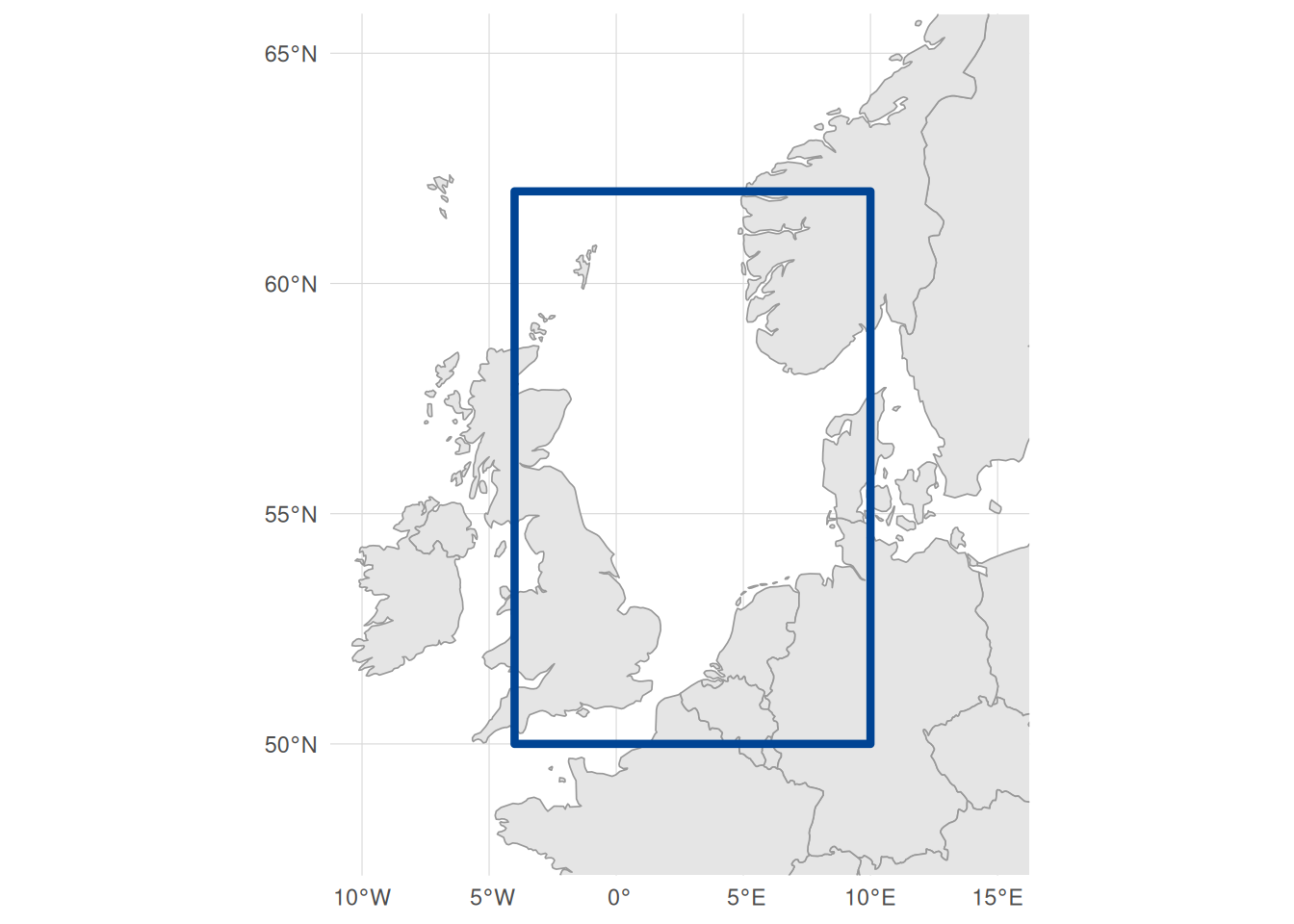
We’ll focus on the North Sea, where UK Essential Fish Habitat data overlaps with EMODnet Biology copepod coverage:
Note that unlike WFS queries (which use a character string like "xmin,ymin,xmax,ymax"), WCS queries in emodnet.wcs expect a named numeric vector with xmin, ymin, xmax, and ymax elements. The bbox is assumed to be in WGS84 (EPSG:4326) by default, but you can specify a different CRS using the crs argument.
Exploring EMODnet WCS Services
Before downloading raster data, let’s explore what’s available.
Discovering Available Services
EMODnet provides raster data through several thematic WCS services:
emdn_wcs()| service_name | service_url |
|---|---|
| bathymetry | https://ows.emodnet-bathymetry.eu/wcs |
| biology | https://geo.vliz.be/geoserver/Emodnetbio/wcs |
| human_activities | https://ows.emodnet-humanactivities.eu/wcs |
| seabed_habitats | https://ows.emodnet-seabedhabitats.eu/geoserver/emodnet_open_maplibrary/wcs |
For this tutorial, we’ll use the biology service for copepod data and the seabed_habitats service for spawning ground predictions.
Connecting to Services
To query a WCS service, we first create client connections:
bio_wcs <- emdn_init_wcs_client(service = "biology")
habitat_wcs <- emdn_init_wcs_client(service = "seabed_habitats")
Discovering Copepod Coverages
Let’s explore what copepod data is available:
bio_coverage_ids <- emdn_get_coverage_ids(bio_wcs)
bio_coverage_ids
#>  [1] "Emodnetbio__ratio_large_to_small_19582016_L1_err"
#>  [2] "Emodnetbio__aca_spp_19582016_L1"
#>  [3] "Emodnetbio__cal_fin_19582016_L1_err"
#>  [4] "Emodnetbio__cal_hel_19582016_L1_err"
#>  [5] "Emodnetbio__met_luc_19582016_L1_err"
#>  [6] "Emodnetbio__oit_spp_19582016_L1_err"
#>  [7] "Emodnetbio__tem_lon_19582016_L1_err"
#>  [8] "Emodnetbio__chli_19582016_L1_err"
#>  [9] "Emodnetbio__tot_lar_19582016_L1_err"
#> [10] "Emodnetbio__tot_sma_19582016_L1_err"
The coverage IDs follow a naming convention:
-
Emodnetbio__prefix indicates EMODnet Biology - Species abbreviation (e.g.,
cal_finfor Calanus finmarchicus) - Time period (
19582016= 1958-2016) - Processing level (e.g.,
L1for the DIVAnd interpolation model) -
_errsuffix indicates error bands are included
For this tutorial, we’ll use four copepod layers that are ecologically relevant for gadoid larvae: Calanus finmarchicus (a key prey species), Temora longicornis (an important coastal copepod), and total large and small copepod relative abundance.
These copepod layers are from EMODnet’s OOPS products, created by interpolating Continuous Plankton Recorder (CPR) survey data using DIVAnd.
The underlying CPR data records organisms per 3 m³ of filtered seawater (from 10 nautical mile tows). However, the DIVAnd interpolation produces dimensionless relative abundance indices rather than absolute counts. Importantly, DIVAnd processes each species independently (univariate analysis), so values are not comparable between species. You can compare spatial patterns within a species (e.g., “Calanus is more abundant here than there”) but not across species (e.g., “Calanus is more abundant than Temora”).
The _err suffix indicates coverages include both relative abundance and error bands.
Understanding Coverage Properties
Let’s examine the metadata for our selected copepod layers:
copepod_ids <- c(
  "Emodnetbio__cal_fin_19582016_L1_err",
  "Emodnetbio__tem_lon_19582016_L1_err",
  "Emodnetbio__tot_lar_19582016_L1_err",
  "Emodnetbio__tot_sma_19582016_L1_err"
)
The emdn_get_coverage_info() function provides a full overview of coverage metadata:
copepod_info <- emdn_get_coverage_info(
  wcs = bio_wcs,
  coverage_ids = copepod_ids
)| data_source | service_name | service_url | coverage_id | band_description | band_uom | constraint | nil_value | dim_n | dim_names | grid_size | resolution | extent | crs | wgs84_extent | temporal_extent | vertical_extent | subtype | fn_seq_rule | fn_start_point | fn_axis_order |
|---|---|---|---|---|---|---|---|---|---|---|---|---|---|---|---|---|---|---|---|---|
| emodnet_wcs | https://geo.vliz.be/geoserver/Emodnetbio/wcs | biology | Emodnetbio__cal_fin_19582016_L1_err | Relative abundance, Relative error | W.m-2.Sr-1 | -3.4028235e+38-3.4028235e+38 | 9.96921e+36 | 3 | lat(deg):geographic; long(deg):geographic; time(s):temporal | 951x401 | 0.1 Deg x 0.1 Deg | -75.05, 34.95, 20.05, 75.05 | EPSG:4326 | -75.05, 34.95, 20.05, 75.05 | 1958-02-16T01:00:00 - 2016-11-16T01:00:00 | NA | RectifiedGridCoverage | Linear | 0,0 | +2,+1 |
| emodnet_wcs | https://geo.vliz.be/geoserver/Emodnetbio/wcs | biology | Emodnetbio__tem_lon_19582016_L1_err | Relative abundance, Relative error | W.m-2.Sr-1 | -3.4028235e+38-3.4028235e+38 | 9.96921e+36 | 3 | lat(deg):geographic; long(deg):geographic; time(s):temporal | 951x401 | 0.1 Deg x 0.1 Deg | -75.05, 34.95, 20.05, 75.05 | EPSG:4326 | -75.05, 34.95, 20.05, 75.05 | 1958-02-16T01:00:00 - 2016-11-16T01:00:00 | NA | RectifiedGridCoverage | Linear | 0,0 | +2,+1 |
| emodnet_wcs | https://geo.vliz.be/geoserver/Emodnetbio/wcs | biology | Emodnetbio__tot_lar_19582016_L1_err | Relative abundance, Relative error | W.m-2.Sr-1 | -3.4028235e+38-3.4028235e+38 | 9.96921e+36 | 3 | lat(deg):geographic; long(deg):geographic; time(s):temporal | 951x401 | 0.1 Deg x 0.1 Deg | -75.05, 34.95, 20.05, 75.05 | EPSG:4326 | -75.05, 34.95, 20.05, 75.05 | 1958-02-16T01:00:00 - 2016-11-16T01:00:00 | NA | RectifiedGridCoverage | Linear | 0,0 | +2,+1 |
| emodnet_wcs | https://geo.vliz.be/geoserver/Emodnetbio/wcs | biology | Emodnetbio__tot_sma_19582016_L1_err | Relative abundance, Relative error | W.m-2.Sr-1 | -3.4028235e+38-3.4028235e+38 | 9.96921e+36 | 3 | lat(deg):geographic; long(deg):geographic; time(s):temporal | 951x401 | 0.1 Deg x 0.1 Deg | -75.05, 34.95, 20.05, 75.05 | EPSG:4326 | -75.05, 34.95, 20.05, 75.05 | 1958-02-16T01:00:00 - 2016-11-16T01:00:00 | NA | RectifiedGridCoverage | Linear | 0,0 | +2,+1 |
To retrieve specific pieces of metadata, we can get a coverage summary object and use accessor functions. For example, let’s examine what dimensions are available for the Calanus coverage:
# Returns a list with one element per coverage ID - extract the first (and only) element
calanus_summary <- emdn_get_coverage_summaries(bio_wcs, copepod_ids[1])[[1]]

# What dimensions does this coverage have?
emdn_get_dimensions_info(calanus_summary, format = "tibble")
The coverage has latitude, longitude, and a time dimension. The range column shows the temporal extent, but to see the actual available time steps we use emdn_get_coverage_dim_coefs():
# Returns a named list - extract the vector for our coverage
time_steps <- emdn_get_coverage_dim_coefs(bio_wcs, copepod_ids[1])[[1]]

# Temporal extent
range(time_steps)
#> [1] "1958-02-16T01:00:00" "2016-11-16T01:00:00"

# How many time steps?
length(time_steps)
#> [1] 236

# Show first few to see the pattern
head(time_steps, 8)
#> [1] "1958-02-16T01:00:00" "1958-05-16T01:00:00" "1958-08-16T01:00:00"
#> [4] "1958-11-16T01:00:00" "1959-02-16T01:00:00" "1959-05-16T01:00:00"
#> [7] "1959-08-16T01:00:00" "1959-11-16T01:00:00"
The 236 timestamps show quarterly data (February, May, August, November) from 1958 to 2016.
We can also check spatial properties:
# Spatial resolution (degrees)
emdn_get_resolution(calanus_summary)
#>   x   y
#> 0.1 0.1
#> attr(,"uom")
#> [1] "Deg" "Deg"

# Bounding box in WGS84
emdn_get_WGS84bbox(calanus_summary)
#>   xmin   ymin   xmax   ymax
#> -75.05  34.95  20.05  75.05
The resolution is 0.1° (approximately 7-11 km depending on latitude). The bounding box spans the North Atlantic, but note that this shows the grid boundaries, not where actual data exists. CPR survey coverage is patchy in some regions, so always check for NA values when working with a specific area.
And band metadata:
# Band descriptions
emdn_get_band_descriptions(calanus_summary)
#> [1] "Relative abundance" "Relative error"
#> attr(,"uom")
#> [1] "W.m-2.Sr-1" "W.m-2.Sr-1"

# Band units of measurement
emdn_get_band_uom(calanus_summary)
#> Relative abundance     Relative error
#>       "W.m-2.Sr-1"       "W.m-2.Sr-1"
The band descriptions confirm these coverages contain two bands: the relative abundance estimate and its error. However, the band_uom shows W.m-2.Sr-1, a radiance unit from remote sensing. This is incorrect metadata, likely propagated from satellite-derived environmental inputs used in the DIVAnd interpolation. As noted above, the actual values are dimensionless relative abundance indices.
Discovering Spawning Ground Coverages
Now let’s find fish spawning ground data that overlaps with our copepod coverage. First, we search for spawning-related coverages:
habitat_coverage_ids <- emdn_get_coverage_ids(habitat_wcs)

# Filter for spawning ground coverages
spawning_ids <- habitat_coverage_ids[grepl(
  "spawning",
  habitat_coverage_ids,
  ignore.case = TRUE
)]
spawning_ids
#>  [1] "emodnet_open_maplibrary__DK004008_EFH_Cod_Spawning grounds"
#>  [2] "emodnet_open_maplibrary__DK004011_EFH_Plaice_Spawning grounds"
#>  [3] "emodnet_open_maplibrary__DK004017_EFH_Flounder_Spawning grounds"
#>  [4] "emodnet_open_maplibrary__FR005109_EFH_Seabass_SpawningGrounds"
#>  [5] "emodnet_open_maplibrary__FR005110_EFH_Dragonets_SpawningGrounds"
#>  [6] "emodnet_open_maplibrary__FR005111_EFH_Cod_SpawningGrounds"
#>  [7] "emodnet_open_maplibrary__FR005112_EFH_Dab_SpawningGrounds"
#>  [8] "emodnet_open_maplibrary__FR005113_EFH_Rocklings_SpawningGrounds"
#>  [9] "emodnet_open_maplibrary__FR005114_EFH_Whiting_SpawningGrounds"
#> [10] "emodnet_open_maplibrary__FR005115_EFH_Flounder_SpawningGrounds"
#> [11] "emodnet_open_maplibrary__FR005116_EFH_Plaice_SpawningGrounds"
#> [12] "emodnet_open_maplibrary__FR005117_EFH_Sole_SpawningGrounds"
#> [13] "emodnet_open_maplibrary__GB000050_EFH_Whiting_SpawningGrounds"
#> [14] "emodnet_open_maplibrary__GB000051_EFH_Haddock_SpawningGrounds"
#> [15] "emodnet_open_maplibrary__PT005001_EFH_Sardine_SpawningGrounds"
#> [16] "emodnet_open_maplibrary__PT005002_EFH_Sardine_SpawningGrounds"
#> [17] "emodnet_open_maplibrary__PT005003_EFH_Sardine_SpawningGrounds"
#> [18] "emodnet_open_maplibrary__PT005004_EFH_Sardine_SpawningGrounds"
#> [19] "emodnet_open_maplibrary__PT005005_EFH_Sardine_SpawningGrounds"
#> [20] "emodnet_open_maplibrary__PT005006_EFH_Sardine_SpawningGrounds"
There are spawning ground predictions from Denmark (DK), France (FR), Great Britain (GB), and Portugal (PT). Let’s get their full metadata to get a better understanding of what they contain:
spawning_info_all <- emdn_get_coverage_info(
  wcs = habitat_wcs,
  coverage_ids = spawning_ids
)
spawning_info_all |>
  dplyr::select(coverage_id, wgs84_extent) |>
knitr::kable()| coverage_id | wgs84_extent |
|---|---|
| emodnet_open_maplibrary__DK004008_EFH_Cod_Spawning grounds | 9.52, 54.12, 13.57, 57.97 |
| emodnet_open_maplibrary__DK004011_EFH_Plaice_Spawning grounds | 9.52, 54.12, 13.57, 57.97 |
| emodnet_open_maplibrary__DK004017_EFH_Flounder_Spawning grounds | 9.52, 54.12, 13.57, 57.97 |
| emodnet_open_maplibrary__FR005109_EFH_Seabass_SpawningGrounds | -5.4, 43.5, -1.15, 48 |
| emodnet_open_maplibrary__FR005110_EFH_Dragonets_SpawningGrounds | -0.05, 49.9, 2.54, 51.4 |
| emodnet_open_maplibrary__FR005111_EFH_Cod_SpawningGrounds | 0.04, 49.9, 2.55, 51.4 |
| emodnet_open_maplibrary__FR005112_EFH_Dab_SpawningGrounds | 0.04, 49.9, 2.55, 51.4 |
| emodnet_open_maplibrary__FR005113_EFH_Rocklings_SpawningGrounds | 0.04, 49.9, 2.55, 51.4 |
| emodnet_open_maplibrary__FR005114_EFH_Whiting_SpawningGrounds | 0.04, 49.9, 2.55, 51.4 |
| emodnet_open_maplibrary__FR005115_EFH_Flounder_SpawningGrounds | 0.04, 49.9, 2.55, 51.4 |
| emodnet_open_maplibrary__FR005116_EFH_Plaice_SpawningGrounds | 0.04, 49.9, 2.55, 51.4 |
| emodnet_open_maplibrary__FR005117_EFH_Sole_SpawningGrounds | 0.04, 49.9, 2.55, 51.4 |
| emodnet_open_maplibrary__GB000050_EFH_Whiting_SpawningGrounds | -4.21, 49.31, 10.07, 61.99 |
| emodnet_open_maplibrary__GB000051_EFH_Haddock_SpawningGrounds | -4.21, 49.31, 10.07, 61.99 |
| emodnet_open_maplibrary__PT005001_EFH_Sardine_SpawningGrounds | -9.95, 35.8, -5.95, 42.05 |
| emodnet_open_maplibrary__PT005002_EFH_Sardine_SpawningGrounds | -9.95, 35.8, -5.95, 42.05 |
| emodnet_open_maplibrary__PT005003_EFH_Sardine_SpawningGrounds | -9.95, 35.8, -5.95, 42.05 |
| emodnet_open_maplibrary__PT005004_EFH_Sardine_SpawningGrounds | -9.95, 35.8, -5.95, 42.05 |
| emodnet_open_maplibrary__PT005005_EFH_Sardine_SpawningGrounds | -9.95, 35.8, -5.95, 42.05 |
| emodnet_open_maplibrary__PT005006_EFH_Sardine_SpawningGrounds | -9.95, 35.8, -5.95, 42.05 |
Checking the spatial extents helps identify which layers might overlap with our North Sea copepod data. Note that wgs84_extent shows grid boundaries, not actual data coverage. When exploring these layers, we found the UK (GB) spawning grounds work best for this tutorial because they cover the North Sea where copepod data is most complete. Other regions had sparse copepod coverage or limited spatial extent.
We’ll use whiting and haddock, both gadoids whose larvae depend on copepods:
spawning_ids <- c(
  "emodnet_open_maplibrary__GB000050_EFH_Whiting_SpawningGrounds",
  "emodnet_open_maplibrary__GB000051_EFH_Haddock_SpawningGrounds"
)
Let’s subset the overall metadata table for the coverages of interest to take a closer look:
| data_source | service_name | service_url | coverage_id | band_description | band_uom | constraint | nil_value | dim_n | dim_names | grid_size | resolution | extent | crs | wgs84_extent | temporal_extent | vertical_extent | subtype | fn_seq_rule | fn_start_point | fn_axis_order |
|---|---|---|---|---|---|---|---|---|---|---|---|---|---|---|---|---|---|---|---|---|
| emodnet_wcs | https://ows.emodnet-seabedhabitats.eu/geoserver/emodnet_open_maplibrary/wcs | seabed_habitats | emodnet_open_maplibrary__GB000050_EFH_Whiting_SpawningGrounds | GRAY_INDEX | W.m-2.Sr-1 | -3.4028235e+38-3.4028235e+38 | NaN | 2 | x(m):geographic; y(m):geographic | 291x399 | 6330.76101732992 m x 5462.12992866693 m | -468141.27, 6327797.09, 1120879.74, 8856763.25 | EPSG:3857 | -4.21, 49.31, 10.07, 61.99 | NA | NA | RectifiedGridCoverage | Linear | 0,0 | +1,+2 |
| emodnet_wcs | https://ows.emodnet-seabedhabitats.eu/geoserver/emodnet_open_maplibrary/wcs | seabed_habitats | emodnet_open_maplibrary__GB000051_EFH_Haddock_SpawningGrounds | GRAY_INDEX | W.m-2.Sr-1 | -3.4028235e+38-3.4028235e+38 | NaN | 2 | x(m):geographic; y(m):geographic | 291x399 | 6330.76101732992 m x 5462.12992866693 m | -468141.27, 6327797.09, 1120879.74, 8856763.25 | EPSG:3857 | -4.21, 49.31, 10.07, 61.99 | NA | NA | RectifiedGridCoverage | Linear | 0,0 | +1,+2 |
The full metadata for our selected layers is in the table above. Key points for combining with our copepod data:
- Resolution: ~6.3 km (finer than the copepod grid at ~10 km)
- Temporal extent: NA, meaning these are static layers with no time dimension, unlike our quarterly copepod data
- Dimensions: Only 2 (x, y), so no time slicing needed when downloading
- CRS: Projected coordinate system (meters), which we’ll need to reproject to match the copepod WGS84 grid
These Essential Fish Habitat (EFH) layers are from the Scottish Government EFH mapping project, produced using decision tree models with fish survey data (2010-2020) and environmental predictors. Environmental predictors include physical oceanographic variables (temperature, depth, salinity, currents) rather than biological factors like prey availability. Values represent habitat suitability (0-1 probability scores).
Again, band_uom shows W.m-2.Sr-1. As with the copepod layers, this likely propagated from satellite-derived environmental inputs used in the models. The actual values are dimensionless suitability scores.
Retrieving Copepod Data
Now, let’s go ahead and start downloading actual data. Let’s start with copepod relative abundance data for the spawning period.
Selecting the Time Period
The copepod data uses quarterly timesteps (February, May, August, November). Gadoids in the North Sea typically spawn in late winter to early spring, so we’ll use February timesteps.
Rather than using a single year (which might be anomalous), we’ll download multiple years and calculate the mean. This gives a more representative picture of typical conditions. We’ll use the three most recent February timesteps available in the dataset (2014-2016):
# Most recent February timesteps available
spawning_times <- c(
  "2014-02-16T01:00:00",
  "2015-02-16T01:00:00",
  "2016-02-16T01:00:00"
)
Downloading Copepod Layers
We can pass multiple time values to emdn_get_coverage() which will return a multi-layer stack.
We’ve seen that these coverages include both relative abundance estimates and associated errors (from the DIVAnd interpolation). In a full analysis, you’d want to consider these errors, as areas with sparse CPR sampling will have higher uncertainty. For simplicity, in this tutorial we’ll focus on the relative abundance values only and use argument rangesubset to request just the “Relative abundance” band from each coverage:
# Download Calanus with all three timepoints, relative abundance band only
calanus_stack <- emdn_get_coverage(
  wcs = bio_wcs,
  coverage_id = "Emodnetbio__cal_fin_19582016_L1_err",
  bbox = north_sea_bbox,
  time = spawning_times,
  rangesubset = "Relative abundance"
)
#> <GMLEnvelope>
#> ....|-- lowerCorner: 50 -4 "1958-02-16T01:00:00"
#> ....|-- upperCorner: 62 10 "2016-11-16T01:00:00"<GMLEnvelope>
#> ....|-- lowerCorner: 50 -4 "1958-02-16T01:00:00"
#> ....|-- upperCorner: 62 10 "2016-11-16T01:00:00"<GMLEnvelope>
#> ....|-- lowerCorner: 50 -4 "1958-02-16T01:00:00"
#> ....|-- upperCorner: 62 10 "2016-11-16T01:00:00"

# Check the structure - one layer per timepoint
calanus_stack
#> class       : SpatRaster
#> size        : 120, 140, 3  (nrow, ncol, nlyr)
#> resolution  : 0.1, 0.1  (x, y)
#> extent      : -4.05, 9.95, 49.95, 61.95  (xmin, xmax, ymin, ymax)
#> coord. ref. : lon/lat WGS 84 (EPSG:4326)
#> sources     : Emodnetbio__cal_fin_19582016_L1_err_2014-02-16T01_00_00_50,-4,62,10.tif
#>               Emodnetbio__cal_fin_19582016_L1_err_2015-02-16T01_00_00_50,-4,62,10.tif
#>               Emodnetbio__cal_fin_19582016_L1_err_2016-02-16T01_00_00_50,-4,62,10.tif
#> names       : Emodnetbio~-abundance, Emodnetbio~-abundance, Emodnetbio~-abundance
Let’s download the remaining copepod layers the same way:
temora_stack <- emdn_get_coverage(
  wcs = bio_wcs,
  coverage_id = "Emodnetbio__tem_lon_19582016_L1_err",
  bbox = north_sea_bbox,
  time = spawning_times,
  rangesubset = "Relative abundance"
)
#> <GMLEnvelope>
#> ....|-- lowerCorner: 50 -4 "1958-02-16T01:00:00"
#> ....|-- upperCorner: 62 10 "2016-11-16T01:00:00"<GMLEnvelope>
#> ....|-- lowerCorner: 50 -4 "1958-02-16T01:00:00"
#> ....|-- upperCorner: 62 10 "2016-11-16T01:00:00"<GMLEnvelope>
#> ....|-- lowerCorner: 50 -4 "1958-02-16T01:00:00"
#> ....|-- upperCorner: 62 10 "2016-11-16T01:00:00"

tot_large_stack <- emdn_get_coverage(
  wcs = bio_wcs,
  coverage_id = "Emodnetbio__tot_lar_19582016_L1_err",
  bbox = north_sea_bbox,
  time = spawning_times,
  rangesubset = "Relative abundance"
)
#> <GMLEnvelope>
#> ....|-- lowerCorner: 50 -4 "1958-02-16T01:00:00"
#> ....|-- upperCorner: 62 10 "2016-11-16T01:00:00"<GMLEnvelope>
#> ....|-- lowerCorner: 50 -4 "1958-02-16T01:00:00"
#> ....|-- upperCorner: 62 10 "2016-11-16T01:00:00"<GMLEnvelope>
#> ....|-- lowerCorner: 50 -4 "1958-02-16T01:00:00"
#> ....|-- upperCorner: 62 10 "2016-11-16T01:00:00"

tot_small_stack <- emdn_get_coverage(
  wcs = bio_wcs,
  coverage_id = "Emodnetbio__tot_sma_19582016_L1_err",
  bbox = north_sea_bbox,
  time = spawning_times,
  rangesubset = "Relative abundance"
)
#> <GMLEnvelope>
#> ....|-- lowerCorner: 50 -4 "1958-02-16T01:00:00"
#> ....|-- upperCorner: 62 10 "2016-11-16T01:00:00"<GMLEnvelope>
#> ....|-- lowerCorner: 50 -4 "1958-02-16T01:00:00"
#> ....|-- upperCorner: 62 10 "2016-11-16T01:00:00"<GMLEnvelope>
#> ....|-- lowerCorner: 50 -4 "1958-02-16T01:00:00"
#> ....|-- upperCorner: 62 10 "2016-11-16T01:00:00"map()
The repetitive download code above could be condensed using purrr::map(). This returns a list of rasters:
copepod_stacks <- map(copepod_ids, \(id) {
  emdn_get_coverage(
    wcs = bio_wcs,
    coverage_id = id,
    bbox = north_sea_bbox,
    time = spawning_times,
    rangesubset = "Relative abundance"
  )
})
We use the explicit approach in this tutorial for clarity, but map() is useful when downloading many coverages.
Averaging Across Years
Each stack now contains three rasters, one for each February (2014, 2015, 2016). To create a representative picture of typical spawning-season conditions, we calculate the mean across years using terra::mean(). This operates cell-by-cell across the stack.
We can use map() to apply the averaging to all stacks at once, then combine the resulting list of rasters into a single multi-layer raster using rast():
# Average across years for each species, then combine into one raster
copepods <- list(
  calanus_stack,
  temora_stack,
  tot_large_stack,
  tot_small_stack
) |>
  map(\(stack) mean(stack, na.rm = TRUE)) |>
  rast()

# Name the layers for easy subsetting and plot labels
names(copepods) <- c("Calanus", "Temora", "Large", "Small")

# Check result - a 4-layer raster
copepods
#> class       : SpatRaster
#> size        : 120, 140, 4  (nrow, ncol, nlyr)
#> resolution  : 0.1, 0.1  (x, y)
#> extent      : -4.05, 9.95, 49.95, 61.95  (xmin, xmax, ymin, ymax)
#> coord. ref. : lon/lat WGS 84 (EPSG:4326)
#> source(s)   : memory
#> names       :    Calanus,     Temora,       Large,      Small
#> min values  : -0.2106529, -0.1512153, -0.09880921, -0.2196849
#> max values  :  2.0994925,  2.4651998,  2.84098649,  5.8262204
The result is a multi-layer SpatRaster where each layer contains the 3-year February mean relative abundance for one copepod type. Note that combining the rasters only works because all four coverages share the same grid (extent and resolution), which they do here as they were produced together as part of the same data product.
Both rast() and c() can combine SpatRaster objects into a multi-layer raster:
-
rast(list_of_rasters)- takes a list of rasters (useful aftermap()) -
c(r1, r2, r3)- takes individual raster objects
For example, if we had individual raster objects instead of a list:
copepods <- c(calanus_mean, temora_mean, large_mean, small_mean)We can check the number of layers and subset using list-like syntax:
# Number of layers
nlyr(copepods)
#> [1] 4

# Subset by name
copepods[["Calanus"]]
#> class       : SpatRaster
#> size        : 120, 140, 1  (nrow, ncol, nlyr)
#> resolution  : 0.1, 0.1  (x, y)
#> extent      : -4.05, 9.95, 49.95, 61.95  (xmin, xmax, ymin, ymax)
#> coord. ref. : lon/lat WGS 84 (EPSG:4326)
#> source(s)   : memory
#> name        :    Calanus
#> min value   : -0.2106529
#> max value   :  2.0994925
copepods$Calanus # equivalent
#> class       : SpatRaster
#> size        : 120, 140, 1  (nrow, ncol, nlyr)
#> resolution  : 0.1, 0.1  (x, y)
#> extent      : -4.05, 9.95, 49.95, 61.95  (xmin, xmax, ymin, ymax)
#> coord. ref. : lon/lat WGS 84 (EPSG:4326)
#> source(s)   : memory
#> name        :    Calanus
#> min value   : -0.2106529
#> max value   :  2.0994925

# Subset by index
copepods[[1]]
#> class       : SpatRaster
#> size        : 120, 140, 1  (nrow, ncol, nlyr)
#> resolution  : 0.1, 0.1  (x, y)
#> extent      : -4.05, 9.95, 49.95, 61.95  (xmin, xmax, ymin, ymax)
#> coord. ref. : lon/lat WGS 84 (EPSG:4326)
#> source(s)   : memory
#> name        :    Calanus
#> min value   : -0.2106529
#> max value   :  2.0994925

# Subset multiple layers
copepods[[c("Calanus", "Temora")]]
#> class       : SpatRaster
#> size        : 120, 140, 2  (nrow, ncol, nlyr)
#> resolution  : 0.1, 0.1  (x, y)
#> extent      : -4.05, 9.95, 49.95, 61.95  (xmin, xmax, ymin, ymax)
#> coord. ref. : lon/lat WGS 84 (EPSG:4326)
#> source(s)   : memory
#> names       :    Calanus,     Temora
#> min values  : -0.2106529, -0.1512153
#> max values  :  2.0994925,  2.4651998
Quick Visualization
Let’s visualize our copepod data. We use tidyterra::geom_spatraster() which integrates terra rasters with ggplot2. Using facet_wrap(~lyr) creates a separate panel for each layer in the stack:
ggplot() +
  geom_spatraster(data = copepods) +
  facet_wrap(~lyr, ncol = 2) +
  scale_fill_viridis_c(
    name = "Relative\nabundance",
    na.value = "white",
    option = "plasma"
  ) +
  labs(
    title = "Copepod Distributions",
    subtitle = "North Sea, February mean (2014-2016)",
    x = NULL,
    y = NULL
  ) +
  theme_minimal() +
  theme(
    axis.text.x = element_text(size = 8, angle = 45, hjust = 1),
    axis.text.y = element_text(size = 8),
    legend.position = "bottom",
    panel.spacing = unit(0.5, "lines")
  )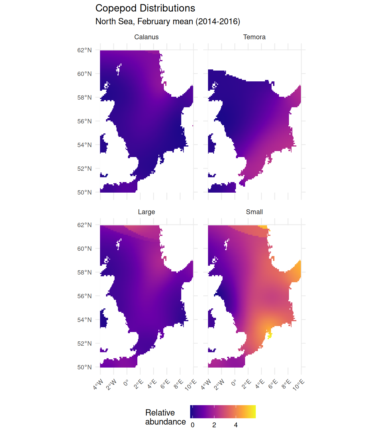
February is relatively early in the seasonal cycle, so values are generally lower than summer months. Each panel shows distinct spatial patterns: total large copepods show higher relative abundance in the northwest, while total small copepods peak in the southeastern North Sea (German Bight) with elevated values extending along the eastern margin. Calanus and Temora both show low values overall, but with contrasting distributions: Calanus peaks in the northwest while Temora is higher in the southeast. Remember that values are not comparable across panels (each species is modelled independently), but the spatial gradients within each layer provide the variation needed for our analysis.
Retrieving Spawning Ground Data
Now let’s download spawning ground predictions for whiting and haddock. With only two coverages, we can use map() to download them in a single step:
# Coverage IDs for each species
spawning_coverage_ids <- c(
  Whiting = "emodnet_open_maplibrary__GB000050_EFH_Whiting_SpawningGrounds",
  Haddock = "emodnet_open_maplibrary__GB000051_EFH_Haddock_SpawningGrounds"
)

# Download each spawning ground layer and combine into a multi-layer raster
spawning <- map(spawning_coverage_ids, \(id) {
  emdn_get_coverage(wcs = habitat_wcs, coverage_id = id, bbox = north_sea_bbox)
}) |>
  rast()
#> <GMLEnvelope>
#> ....|-- lowerCorner: -445277.963173094 6446275.84101716
#> ....|-- upperCorner: 1113194.90793274 8859142.8005657
#> <GMLEnvelope>
#> ....|-- lowerCorner: -445277.963173094 6446275.84101716
#> ....|-- upperCorner: 1113194.90793274 8859142.8005657

spawning
#> class       : SpatRaster
#> size        : 441, 246, 2  (nrow, ncol, nlyr)
#> resolution  : 6330.761, 5462.13  (x, y)
#> extent      : -442818.2, 1114549, 6447964, 8856763  (xmin, xmax, ymin, ymax)
#> coord. ref. : WGS 84 / Pseudo-Mercator (EPSG:3857)
#> sources     : emodnet_open_maplibrary__GB000050_EFH_Whiting_SpawningGrounds_-445277.963173094,6446275.84101716,1113194.90793274,8859142.8005657.tif
#>               emodnet_open_maplibrary__GB000051_EFH_Haddock_SpawningGrounds_-445277.963173094,6446275.84101716,1113194.90793274,8859142.8005657.tif
#> names       : Whiting, Haddock
Defining a Suitability Threshold
To characterize copepod conditions in spawning habitat, we need to classify cells as either suitable or unsuitable spawning grounds. This requires choosing a threshold on the suitability index to divide the data into two zones: areas above the threshold representing functional spawning habitat, and areas below representing marginal or unsuitable habitat.
Habitat suitability indices range from 0 (unsuitable) to 1 (highly suitable), but interpreting intermediate values requires care. We want to exclude low-suitability cells that likely represent poor or marginal habitat. A threshold of 0.3 is commonly used in habitat suitability studies to separate “unsuitable” from “marginal” habitat (Brooks 1997; Kim et al. 2025), so we adopt this value:
suitability_threshold <- 0.3Ideally, thresholds for habitat suitability models would be derived from model training data using statistical methods like “minimum training presence” (the lowest suitability at which the species was observed) or “maximum sum of sensitivity and specificity” (Liu et al. 2005). However, these approaches require access to the original occurrence data and model outputs, which we don’t have for these spawning ground predictions.
When such data aren’t available, common practice provides a pragmatic alternative. Values around 0.3 frequently appear as the boundary between “poor/unsuitable” and “marginal” habitat across various systems, from wildlife assessments (Brooks 1997) to recent plant distribution studies (Kim et al. 2025). We adopt this threshold to focus on areas with at least moderate suitability.
Exploring Spawning Ground Suitability
Let’s examine the distribution of habitat suitability values. We iterate over each layer using map(), extract cell values as a vector with terra::values(), and calculate summary statistics:
# Calculate summary statistics for each species
suitability_summary <- map(names(spawning), \(sp) {
  vals <- spawning[[sp]] |> values() |> na.omit()
  tibble(
    species = sp,
    n = length(vals),
    min = min(vals),
    max = max(vals),
    mean = mean(vals),
    median = median(vals),
    pct_above_threshold = sum(vals > suitability_threshold) / length(vals) * 100
  )
}) |>
  list_rbind()

suitability_summary |>
  mutate(across(where(is.numeric) & !n, ~ round(.x, 3))) |>
  knitr::kable(
    col.names = c(
      "Species",
      "n",
      "Min",
      "Max",
      "Mean",
      "Median",
      paste0("% > ", suitability_threshold)
    ),
    caption = "Spawning ground suitability statistics by species"
)| Species | n | Min | Max | Mean | Median | % > 0.3 |
|---|---|---|---|---|---|---|
| Whiting | 48700 | 0 | 1.000 | 0.219 | 0.143 | 20.877 |
| Haddock | 48259 | 0 | 0.939 | 0.072 | 0.033 | 2.518 |
The two species show markedly different suitability distributions. Whiting spawning grounds have higher mean suitability (0.22 vs 0.07) and a much larger proportion of cells above our threshold (20.9% vs 2.5%). This indicates that the whiting model predicts more extensive suitable habitat, while haddock suitability is concentrated in a smaller area with most cells showing low values.
Visualizing Spawning Grounds
Let’s visualize the spatial distribution of spawning suitability. We use geom_spatraster_contour() to add a contour line at our threshold value, delineating areas of suitable habitat:
ggplot() +
  geom_spatraster(data = spawning) +
  geom_spatraster_contour(
    data = spawning,
    breaks = suitability_threshold,
    color = "white",
    linewidth = 0.3
  ) +
  facet_wrap(~lyr, ncol = 2) +
  scale_fill_viridis_c(
    name = "Habitat\nsuitability",
    na.value = "white",
    option = "mako"
  ) +
  labs(
    title = "Gadoid Spawning Grounds",
    subtitle = paste0(
      "UK Essential Fish Habitat predictions (threshold = ",
      suitability_threshold,
      ")"
    )
  ) +
  theme_minimal() +
  theme(
    axis.text = element_text(size = 7),
    legend.position = "bottom"
  )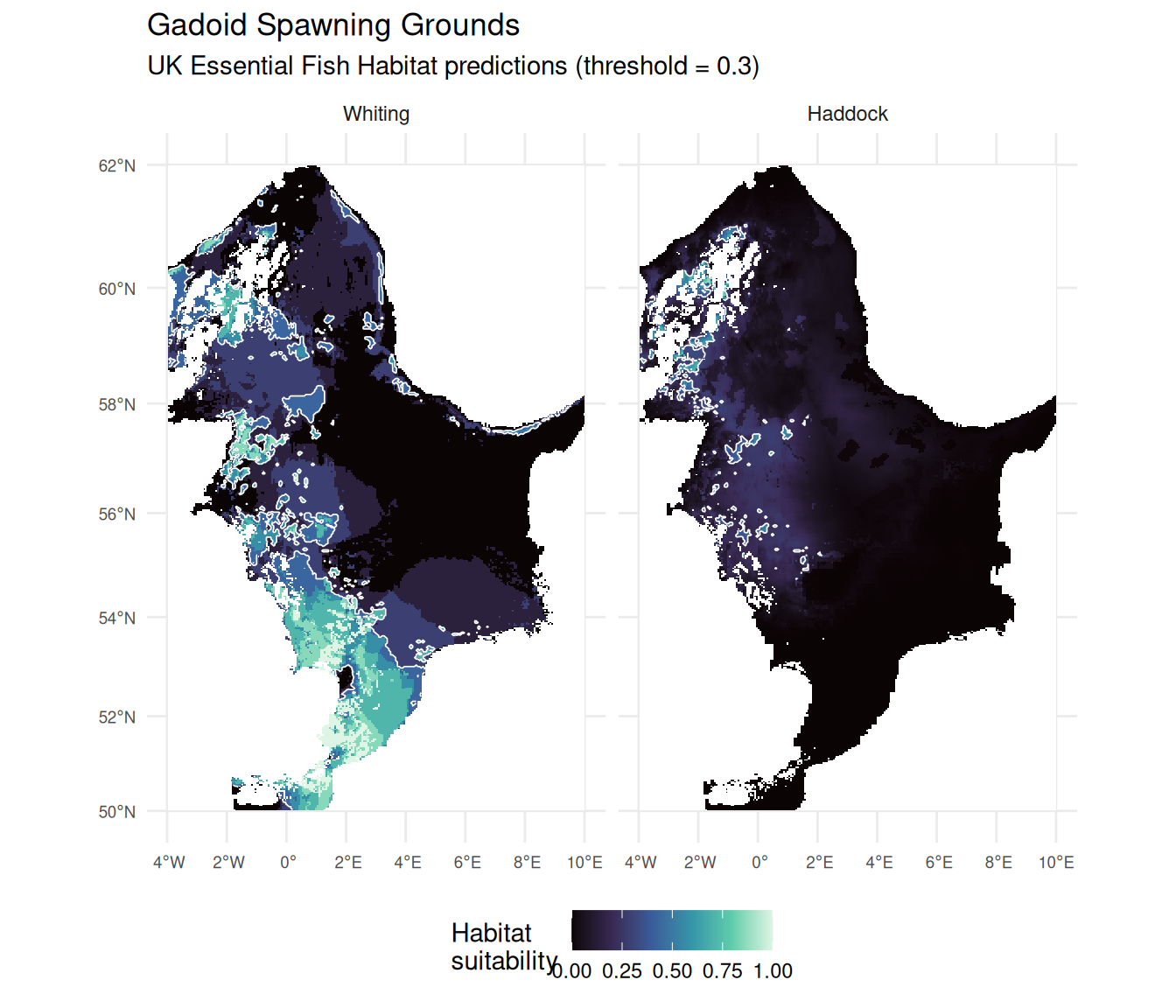
The maps confirm what the statistics suggested: whiting spawning grounds show distinct hotspots (lighter areas) particularly in the western and southern North Sea, while haddock suitability is more uniformly low across the coverage area with only subtle variation in the northern region.
Aligning Rasters for Analysis
To compare copepod and spawning ground data, we need to align them to a common grid. First, let’s check whether alignment is necessary by comparing each raster’s properties. We use terra::res() to check the resolution (cell size), terra::crs() to check the coordinate reference system, and terra::is.lonlat() to check whether the CRS uses geographic coordinates (degrees). By default, crs() returns the full WKT (Well-Known Text) string which is verbose; setting describe = TRUE returns a data frame with parsed CRS details including the name and EPSG code:
The copepods data uses WGS84 (geographic coordinates) while the spawning data uses Web Mercator (EPSG:3857, a projected CRS). The is.lonlat() results confirm that copepods uses degrees while spawning does not - projected CRS typically use meters. This means the resolution values aren’t directly comparable since they’re in different units.
To align the rasters, we need to choose a target grid. Two considerations guide this choice:
Resolution: Best practice is to resample to the coarser resolution to avoid creating artificial detail (see Pebesma and Bivand 2023, Ch. 5). The copepod grid at 0.1° translates to roughly 6-11 km cells at North Sea latitudes, while the spawning grid is approximately 6 km - similar resolutions.
CRS suitability: Web Mercator (EPSG:3857) is designed for web mapping, not spatial analysis - it severely distorts areas at higher latitudes like the North Sea. WGS84, while not ideal for area calculations, avoids this distortion.
Since the resolutions are similar and the copepod data drives our analysis question, we resample spawning to match the copepod grid.
We use terra::project() to reproject the spawning data onto the copepod grid. The first argument is the raster to transform, the second is the target raster (whose CRS, extent, and resolution will be matched), and method specifies the resampling algorithm - "bilinear" interpolates values from the four nearest cells, which is appropriate for continuous data like suitability scores.
In Tutorial 1, we emphasized that vector spatial operations requiring accurate area or distance calculations should use an appropriate projected CRS. For raster analysis, the situation is different.
When we calculate zonal statistics (e.g., mean copepod abundance within spawning areas), we’re averaging cell values - each cell contributes equally regardless of its geographic area. This is appropriate when the underlying data was modeled on the same grid, as the values already represent conditions at that cell’s location.
There is a subtlety: in WGS84, cells don’t represent equal areas - a 0.1° cell near Scotland covers less area than one near the English Channel. For area-weighted analyses or when comparing total quantities across latitudes, this matters. But for our analysis - characterizing typical copepod conditions within spawning grounds - treating cells equally is reasonable, especially within the relatively narrow latitude range of the North Sea (~50-62°N).
Characterizing Copepod Conditions
Now we can extract copepod statistics within each species’ spawning grounds.
Building a Tidy Data Frame
To analyze the relationship between spawning suitability and copepod abundance, we first extract all raster values into a tidy data frame. We combine the aligned spawning and copepod rasters using c(), then use tidyterra::as_tibble() to extract cell values as a tibble with one column per layer:
Now we reshape this wide data frame into tidy (long) format. We use two pivot_longer() calls to create fish and copepod columns, classify cells as above or below our suitability threshold, and finally drop any rows with missing values using drop_na():
cell_data <- cell_values |>
  pivot_longer(
    cols = c(Whiting, Haddock),
    names_to = "fish",
    values_to = "suitability"
  ) |>
  pivot_longer(
    cols = c(Calanus, Temora, Large, Small),
    names_to = "copepod",
    values_to = "abundance"
  ) |>
  mutate(suitable = suitability >= suitability_threshold) |>
  drop_na()

cell_data
Each row now represents one cell-fish-copepod combination, with the suitability value, copepod abundance, and whether the cell exceeds our suitability threshold. The drop_na() removes cells where either the spawning suitability or copepod abundance is missing (NA values in the copepod data indicate areas outside CPR survey coverage).
Summary Statistics
With our tidy data frame, calculating summary statistics by group is straightforward using group_by() and summarise(). We group by fish species, habitat suitability, and copepod type, then calculate the mean and standard deviation of copepod abundance for each combination. The result is reshaped to a wider format for easier reading:
cell_data |>
  # Group by all classification variables
  group_by(fish, suitable, copepod) |>
  # Calculate summary statistics for each group
  summarise(
    mean = mean(abundance),
    sd = sd(abundance),
    n = n(),
    .groups = "drop"
  ) |>
  # Convert logical to readable labels
  mutate(suitable = if_else(suitable, "Suitable", "Unsuitable")) |>
  # Reshape to wide format for display
  select(fish, suitable, copepod, mean) |>
  pivot_wider(names_from = copepod, values_from = mean) |>
  mutate(across(where(is.numeric), ~ round(.x, 3))) |>
  knitr::kable(
    col.names = c("Fish", "Habitat", "Calanus", "Temora", "Large", "Small")
)| Fish | Habitat | Calanus | Temora | Large | Small |
|---|---|---|---|---|---|
| Haddock | Unsuitable | 0.392 | 0.894 | 2.416 | 0.855 |
| Haddock | Suitable | 0.146 | 0.442 | 1.036 | 0.036 |
| Whiting | Unsuitable | 0.435 | 0.939 | 2.459 | 0.825 |
| Whiting | Suitable | 0.230 | 0.700 | 2.174 | 0.897 |
Comparing Suitable vs Unsuitable Habitat
Now that we have our tidy data frame with habitat classifications, we can compare copepod conditions between suitable and unsuitable spawning areas. We reuse the same group_by() and summarise() pattern from the table above, but this time pipe the results directly into ggplot2 for visualization. The bar chart uses geom_col() with position = "dodge" to place bars side-by-side, and geom_errorbar() to show standard deviations. We facet by fish species to compare patterns:
cell_data |>
  group_by(fish, suitable, copepod) |>
  summarise(
    mean = mean(abundance),
    sd = sd(abundance),
    .groups = "drop"
  ) |>
  mutate(suitable = if_else(suitable, "Suitable", "Unsuitable")) |>
  ggplot(aes(x = copepod, y = mean, fill = suitable)) +
  geom_col(position = "dodge") +
  geom_errorbar(
    aes(ymin = mean - sd, ymax = mean + sd),
    position = position_dodge(width = 0.9),
    width = 0.25
  ) +
  facet_wrap(~fish) +
  scale_fill_manual(
    values = c("Suitable" = "#228B22", "Unsuitable" = "grey60"),
    name = "Habitat"
  ) +
  labs(
    title = "Copepod Conditions by Habitat Suitability",
    subtitle = paste0(
      "Mean ± SD relative abundance (threshold = ",
      suitability_threshold,
      ")"
    ),
    x = "Copepod type",
    y = "Mean relative abundance"
  ) +
  theme_minimal() +
  theme(
    axis.text.x = element_text(angle = 45, hjust = 1),
    legend.position = "bottom"
  )
An interesting pattern emerges: unsuitable spawning habitat tends to have higher copepod abundance than suitable habitat. This trend is particularly striking for haddock, where unsuitable areas show substantially higher mean abundance across all copepod types. For whiting, the pattern is similar but less pronounced, with the exception of Temora where suitable habitat actually shows slightly higher abundance. We’ll explore what might explain this in the Discussion.
Exploring the Full Suitability Gradient
The bar chart shows averages, but the relationship between suitability and copepod abundance may be more nuanced. Let’s examine how copepod abundance varies across the full range of suitability values:
ggplot(cell_data, aes(x = suitability, y = abundance, color = fish)) +
  geom_point(alpha = 0.15, size = 0.8) +
  geom_vline(
    xintercept = suitability_threshold,
    linetype = "dashed",
    color = "black",
    linewidth = 0.6
  ) +
  geom_smooth(
    method = "loess",
    se = TRUE,
    color = "grey40",
    fill = "grey80",
    linewidth = 0.8
  ) +
  facet_grid(copepod ~ fish, scales = "free_y") +
  scale_color_manual(values = c("Haddock" = "#E69F00", "Whiting" = "#56B4E9")) +
  labs(
    title = "Spawning Habitat Suitability vs Copepod Abundance",
    x = "Habitat suitability",
    y = "Copepod relative abundance"
  ) +
  theme_minimal() +
  theme(
    strip.text = element_text(size = 9, face = "bold"),
    axis.text = element_text(size = 7),
    legend.position = "none"
  )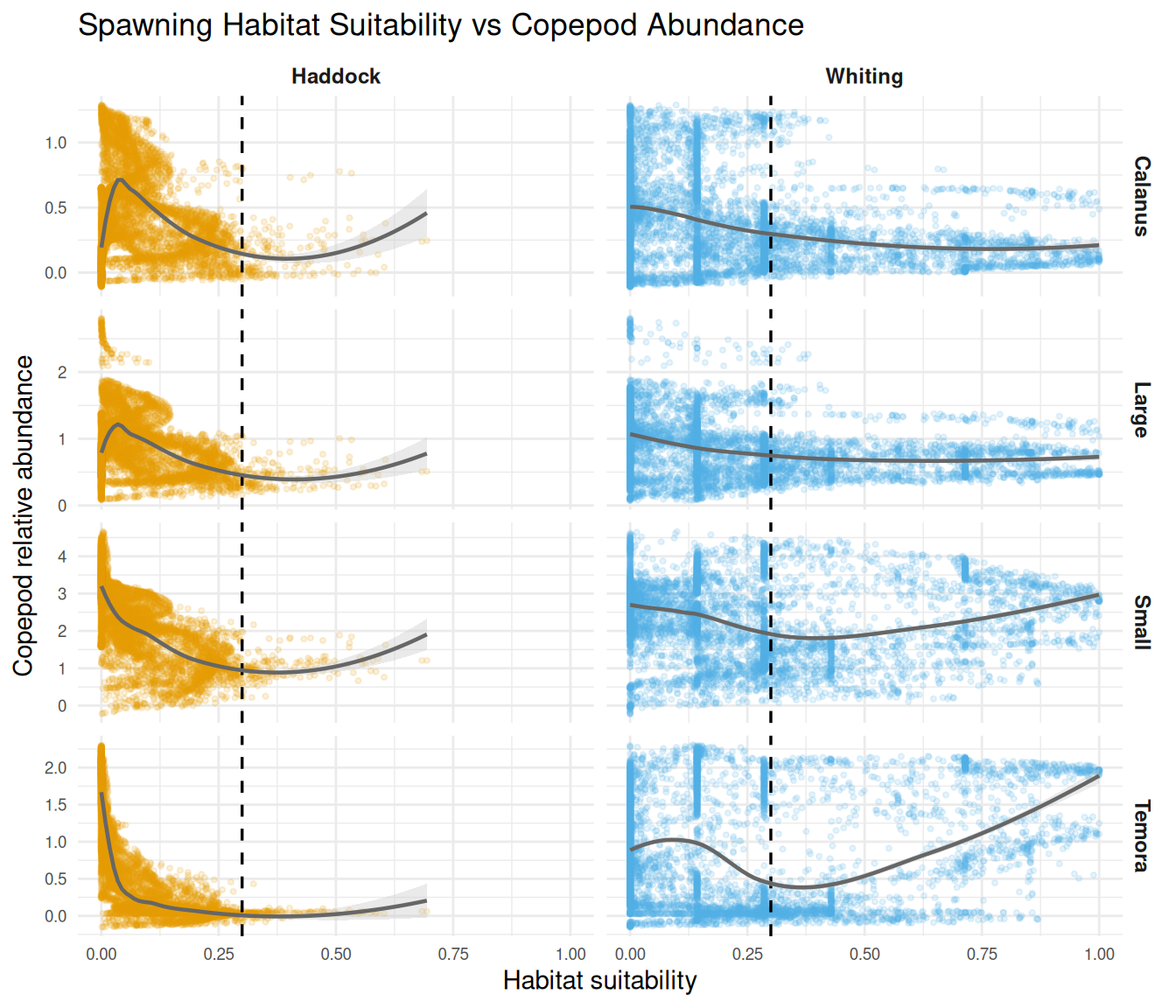
The scatter plots show the full range of variation in the data. The vertical dashed line marks our suitability threshold (0.3). Various patterns are visible - declining trends, flat regions, and even upticks at higher suitability values for some fish-copepod combinations. We interpret these patterns in the Discussion.
Spatial Overlays
Finally, let’s create an interactive map to explore the spatial relationship between copepod abundance and spawning grounds visually. This allows us to see how the copepod distributions align geographically with the predicted spawning areas.
Preparing Spawning Ground Boundaries
First, we need to convert our continuous suitability rasters into polygon boundaries showing “suitable” areas. We create binary masks by applying our threshold, then convert to polygons using terra::as.polygons(). This function creates vector polygons from raster cells, grouping adjacent cells with the same value. We then convert to sf objects and filter to keep only the suitable areas (value = 1):
# Create binary masks: TRUE where suitability >= threshold
whiting_suitable <- spawning_aligned$Whiting >= suitability_threshold
haddock_suitable <- spawning_aligned$Haddock >= suitability_threshold

# Convert raster masks to polygon boundaries
# as.polygons() groups adjacent cells with the same value into polygons
whiting_poly <- as.polygons(whiting_suitable) |>
  st_as_sf() |>
  filter(Whiting == 1)  # Keep only suitable areas

haddock_poly <- as.polygons(haddock_suitable) |>
  st_as_sf() |>
  filter(Haddock == 1)
Building the Interactive Map
We use the tmap package in “view” mode to create an interactive Leaflet map. Maps in tmap are built by combining a tm_shape() call (which specifies the spatial data) with one or more layer functions like tm_raster() or tm_borders() (which specify how to display it). Multiple shapes and layers are combined with +.
The key feature here is layer group controls: by setting group.control = "radio" on each copepod layer, we create mutually exclusive radio buttons that let users switch between copepod types. This avoids visual clutter from overlapping semi-transparent rasters.
The map components are:
-
tm_basemap(): A neutral grey basemap that won’t distract from our data. We setgroup.control = "none"so it doesn’t appear in the layer controls. -
tm_raster(): Each copepod layer with consistent color scaling. Thegroupparameter sets the label shown in the radio button control. The legend title includes both the copepod name and “(relative abundance)” so users always know what they’re viewing. -
tm_borders(): Spawning ground boundaries as polygon outlines. Grey for whiting, cyan for haddock, both always visible (group.control = "none"). -
tm_add_legend(): A manual legend for the spawning ground boundaries, sincetm_borders()with a fixed color doesn’t automatically generate one.
# Switch tmap to interactive (Leaflet) mode
tmap_mode("view")

# Build the map layer by layer
tm_basemap("Esri.WorldGrayCanvas", group.control = "none") +
  # Copepod raster layers with radio button controls
  tm_shape(copepods$Calanus) +
  tm_raster(
    col.scale = tm_scale_continuous(values = "plasma"),
    col.legend = tm_legend(title = "Calanus\n(relative abundance)"),
    group.control = "radio"
  ) +
  tm_shape(copepods$Temora) +
  tm_raster(
    col.scale = tm_scale_continuous(values = "plasma"),
    col.legend = tm_legend(title = "Temora\n(relative abundance)"),
    group.control = "radio"
  ) +
  tm_shape(copepods$Large) +
  tm_raster(
    col.scale = tm_scale_continuous(values = "plasma"),
    col.legend = tm_legend(title = "Large copepods\n(relative abundance)"),
    group = "Large copepods",  # Override default "Large" for clearer label
    group.control = "radio"
  ) +
  tm_shape(copepods$Small) +
  tm_raster(
    col.scale = tm_scale_continuous(values = "plasma"),
    col.legend = tm_legend(title = "Small copepods\n(relative abundance)"),
    group = "Small copepods",  # Override default "Small" for clearer label
    group.control = "radio"
  ) +
  # Spawning ground boundaries (always visible)
  tm_shape(whiting_poly) +
  tm_borders(col = "grey", lwd = 2, group.control = "none") +
  tm_shape(haddock_poly) +
  tm_borders(col = "cyan", lwd = 2, group.control = "none") +
  # Manual legend for spawning ground boundaries
  tm_add_legend(
    type = "lines",
    labels = c("Whiting spawning", "Haddock spawning"),
    col = c("grey", "cyan"),
    lwd = 2,
    title = "Spawning grounds"
)You can pass a multi-layer raster directly to tm_raster():
This creates facets (separate panels for each layer), similar to using facet_wrap() with ggplot2. Here we use separate tm_shape() calls because we want a single map with switchable layers.
Click the layer control icon (stacked squares) in the top right corner to reveal the radio buttons. Select different copepod types to see how their spatial distributions compare to the spawning ground boundaries. You can also zoom and pan to explore specific areas in detail.
Discussion
The clearest pattern from our analysis is that predicted spawning grounds tend to have lower copepod relative abundance compared to unsuitable areas (Figure 4). This pattern is most consistent for Calanus and large copepods across both fish species. Small copepods show weaker differences, and Temora shows a reversed pattern for whiting (slightly higher in suitable areas). The scatter plots (Figure 5) show more varied patterns at finer scales, but these should not be over-interpreted as we performed exploratory analysis only (summaries and visualizations, not formal statistical testing).
Both copepod distributions and spawning suitability show distinct spatial structure in the North Sea. Copepods vary with oceanographic gradients (Calanus higher offshore, Temora and small copepods higher in coastal areas), while spawning suitability reflects physical habitat factors. When two spatially structured variables are overlaid, apparent patterns can emerge from geographic coincidence alone.
This lack of a clear ecological relationship actually makes sense. Adult fish select spawning sites based on physical factors such as temperature, depth, substrate type, and hydrography (González-Irusta and Wright 2016), not prey availability. Copepod abundance matters more for larvae after hatching than for spawning adults. The ecologically relevant question is whether larvae encounter sufficient prey during early development (the “match-mismatch” hypothesis, Endo et al. (2022)), which depends on nursery ground conditions and timing, not spawning site characteristics.
More ecologically relevant analyses (e.g., copepod conditions on nursery grounds) were limited by spatial coverage gaps between available EMODnet datasets.
Despite the limited ecological conclusions, this tutorial successfully demonstrates the technical workflow for combining EMODnet WCS raster layers: accessing multi-dimensional coverages, aligning different resolutions and coordinate systems, building tidy data frames from raster values, and visualizing spatial relationships. These skills transfer directly to analyses where the ecological question and available data are better matched.
What You’ve Learned
This tutorial demonstrated key skills for working with EMODnet raster data:
-
Exploring WCS services: Using
emdn_get_coverage_info()to understand available data - Temporal subsetting: Selecting specific time slices from multi-dimensional coverages
- Multi-source integration: Combining rasters from different EMODnet services
-
Resolution handling: Aligning data with different spatial resolutions using
project() - Zonal statistics: Extracting environmental conditions within habitat areas
- Visualization: Creating informative maps with raster data and contour overlays
These skills transfer to many marine spatial analyses where you need to characterize environmental conditions across habitats or species distributions.
Further Resources
- Continuous Plankton Recorder Survey: www.cprsurvey.org for long-term plankton monitoring with raw data access
- ICES: ices.dk for stock assessments and biological data for North Sea fish
- EMODnet Biology Portal: emodnet.ec.europa.eu/en/biology for additional species distribution products
Ready for more? Continue to Tutorial 3 to learn how to combine WFS vector data with WCS raster data for integrated analyses.